Persistent Homology in Keystroke Recognition

This research project utilizes persistent homology to examine student typing data collected from online proctoring sites and identify trends indicating academic misconduct. Topological data analysis is applied to evaluate the algebraic facets of the persistence of holes in a given space and display high-dimensional data trends.

The following report will explain the general background information behind Persistent Homology, the code used to study different typing patterns, and the results we found.

All code for this project can be found on the following GitHub repository.

What is Persistent Homology?

Generally, Persistent Homology can be defined as an algebraic method for discerning topological features of a space created from a data set. Some examples of topological features are connected components, loops, voids, and simplicial structures, which will be explained in more detail further down.

Let us first consider this point cloud that consists of 19 points in a plane:

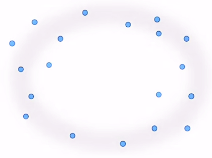
We can see that this data seems to have a general “loop” shape. But how can we quantify the fact that this has a “loop shape”? This is where Persistent Homology comes in.

One idea to quantify the “loop” shape is to connect nearby points. With 0th Persistent Homology, we have balls or spheres simultaneously growing around each point. And as the balls are intersecting, they are forming and merging connected components. This process can be seen more clearly with this diagram, where different colors are assigned to different connected components.

When a ball in one connected component first touches a ball from a different one, the connected components merge and become one bigger connected component. 0th Persistent Homology is the tracking of these connected components.

So, with the previous point cloud, we can see how the balls grow to a diameter of $d$, which is the point when the balls all intersect and merge into one connected component.

As we move forward, it is important to note that the nth homology is quantifying or keeping track of n+1 dimensional holes.

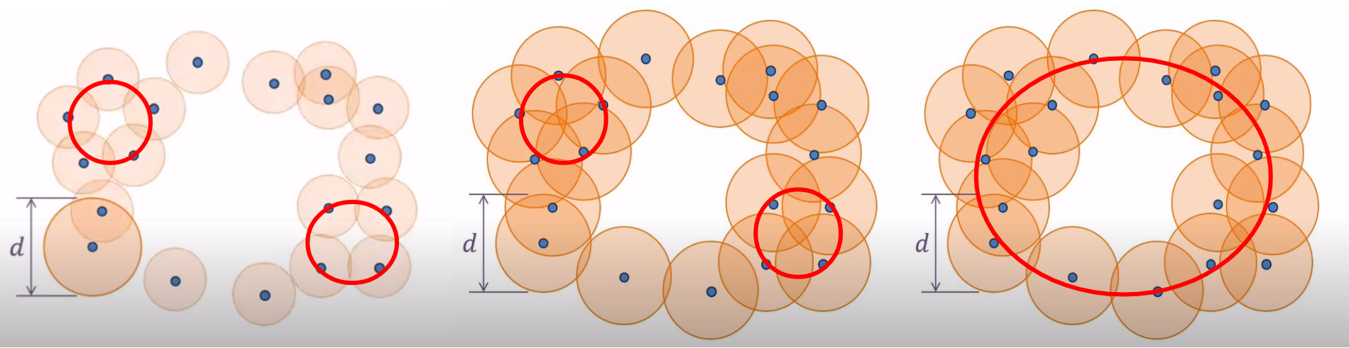
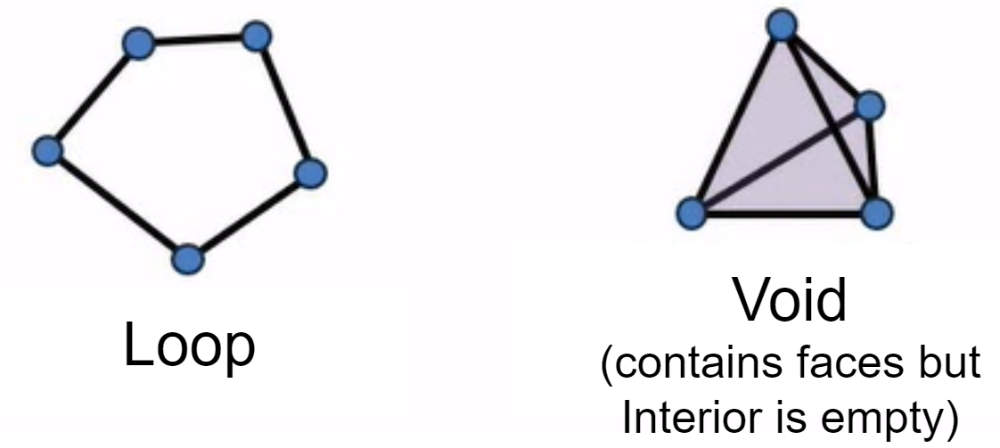
Hence, with 1st Persistent Homology, we still have balls growing simultaneously around the points, but now we are paying attention to the loops that form and disappear as the balls grow. A loop is formed or born when the white space is enclosed around a ring of balls, as seen in the first figure below. As the balls continue to grow, the white space decreases and eventually disappears, being completely filled in by the balls, which we call its death (seen in second figure). However, as the balls grow, a larger loop is also born (seen in third figure) which eventually dies as well.

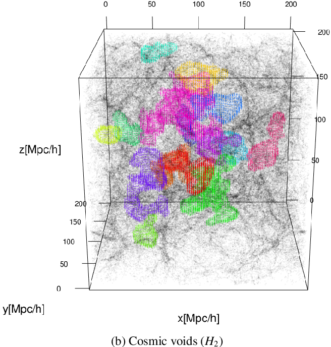
With 2nd Persistent Homology, we are keeping track of voids or cavities which also are born and die as the spheres around each point grow. You can see an example of voids in this diagram:

In simpler terms, we can think of homology as counting these connected components, holes, and voids. But with the figures shown so far, we still are not able to properly compute or quantify anything. So, we introduce simplices.

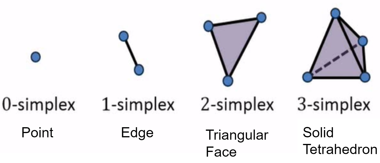
Starting with a zero-dimensional simplex, we have a point. Next, an edge between two points is a one-dimensional simplex. A triangular face is a two-dimensional simplex. A solid tetrahedron is a three-dimensional simplex. And this pattern continues as we go higher in dimensions.

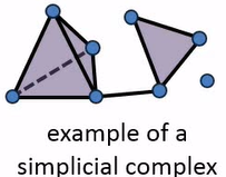
Moreover, if we put together simplices together in a way that the intersection between any two simplices is also a simplex, we obtain a simplicial complex, which you can see an example of below. Hence, simplicial complexes are built from points, lines, and triangular faces. Homology keeps track of the loops and voids present within our simplicial complexes.

     

Now, returning to our original point cloud and applying the simplices, we have this diagram that shows the simplicial complex changing as the balls grow. The simplicial complex allows us to identify and quantify where the holes are computational.

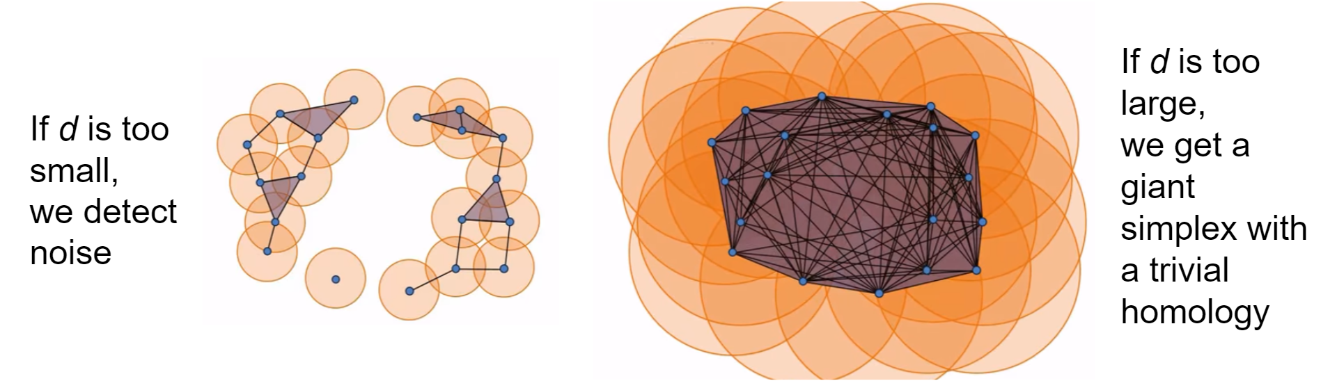
However, we still need to determine the appropriate distance $d$ at which our simplicial complex contains significant features. As seen below, when $d$ is too small, we are only detecting noise and when we choose a $d$ that is too large, we end up with a giant simplex displaying a trivial homology.

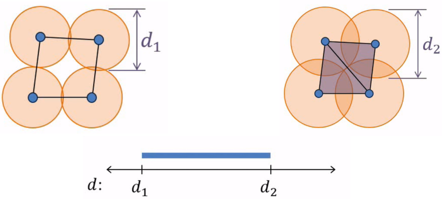
This is where the idea of persistence comes in. In particular, we are interested in studying the birth time and death time of the holes and voids in our simplicial complexes. In the example below, we can see how the barcode on the graph is tracking the distances $d$ at which a loop is born, continuing while it is present, and ending upon the loop’s death.

Now, we can see how this applies to our original point cloud, as the general loop shape shows up in the barcode as the most persistent feature of our data while smaller loops are shown to be less significant and can be deemed as noise.

Moreover, bottleneck distances are the distances between barcodes which we will be using to measure/compare different barcodes.

Of course, as our dimensions grow, it becomes increasingly difficult to create clear visualizations of our data. However, we are still able to carry out the computations because we can use Persistent Homology to quantify the features of our data.

Identifying Keyboard Users Using Persistent Homology

Now that we have covered the basics of persistent homology, we can use this method of topological data analysis to examine student typing data and investigate possible trends of academic misconduct. More specifically, we will be calculating persistence diagrams for all the test subjects in the study, and then identifying each subject using the bottleneck distance of their respective persistence diagrams.

Throughout this section, we will be using the Keystroke Dynamics - Benchmark Data Set which contains a little over 20,000 rows. Each test subject has 8 typing sessions consisting of 50 repetitions in which they retype passwords. The data details how long each key is pressed down and the time between the pressing of each key.

We began by preprocessing the data so that we can generate a persistence diagram for each typing session. To do this, we group the typing data by test subject and store it in a list. We also created a list that contains the corresponding labels. In order to get better results, we shuffle the data before splitting each test subject’s typing data and labels into the 8 sessions. We then created a persistence diagram for each typing session, extracted the persistence intervals in the specified dimensions, and generated our training and testing data to use in a k-nearest neighbors classifier.

Next, we created Vietoris-Rips complexes and their respective simplex trees for each subject’s typing data, and then we calculate the persistence. Due to our hardware limitations, we only compute the first three homologies at a maximum edge length of 0.8.

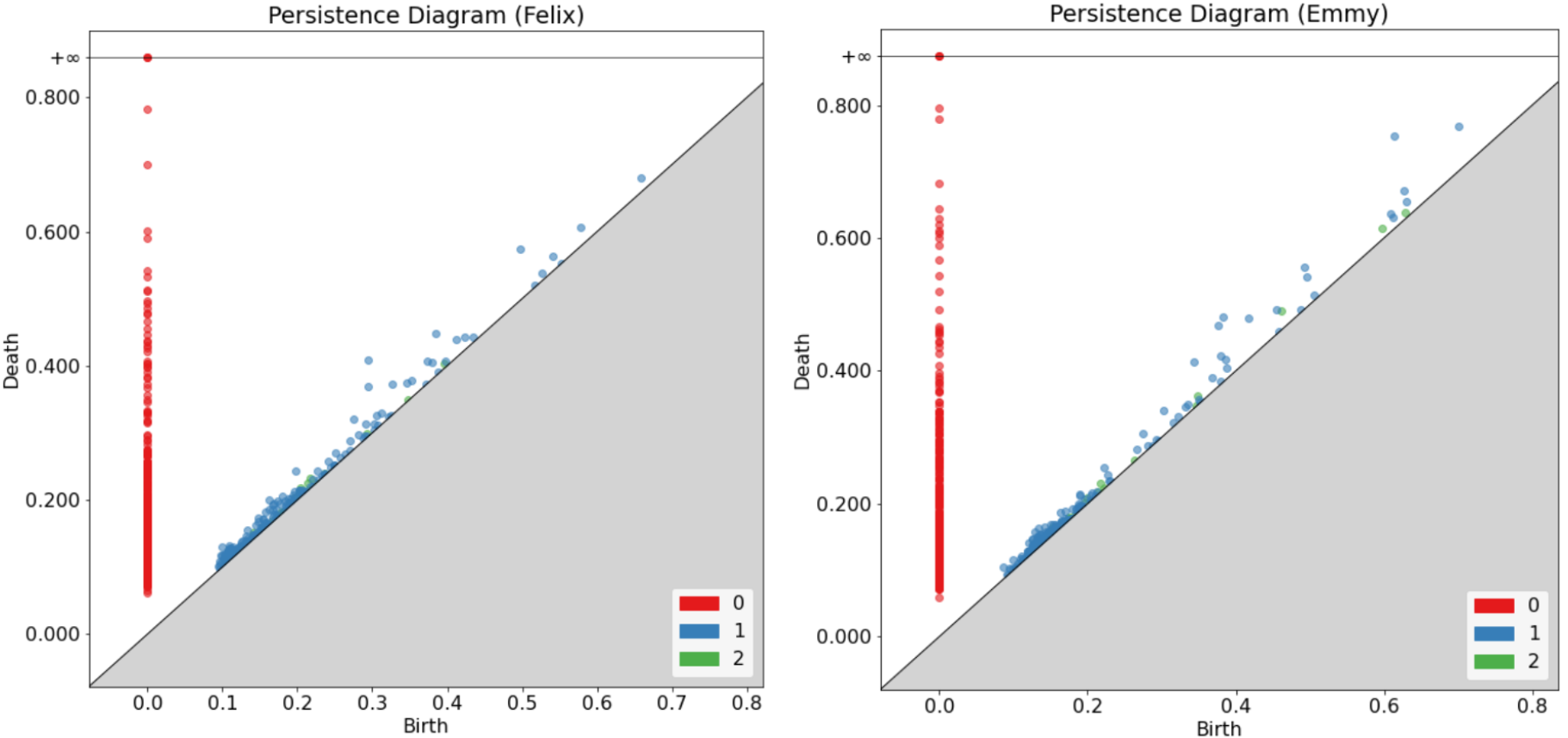
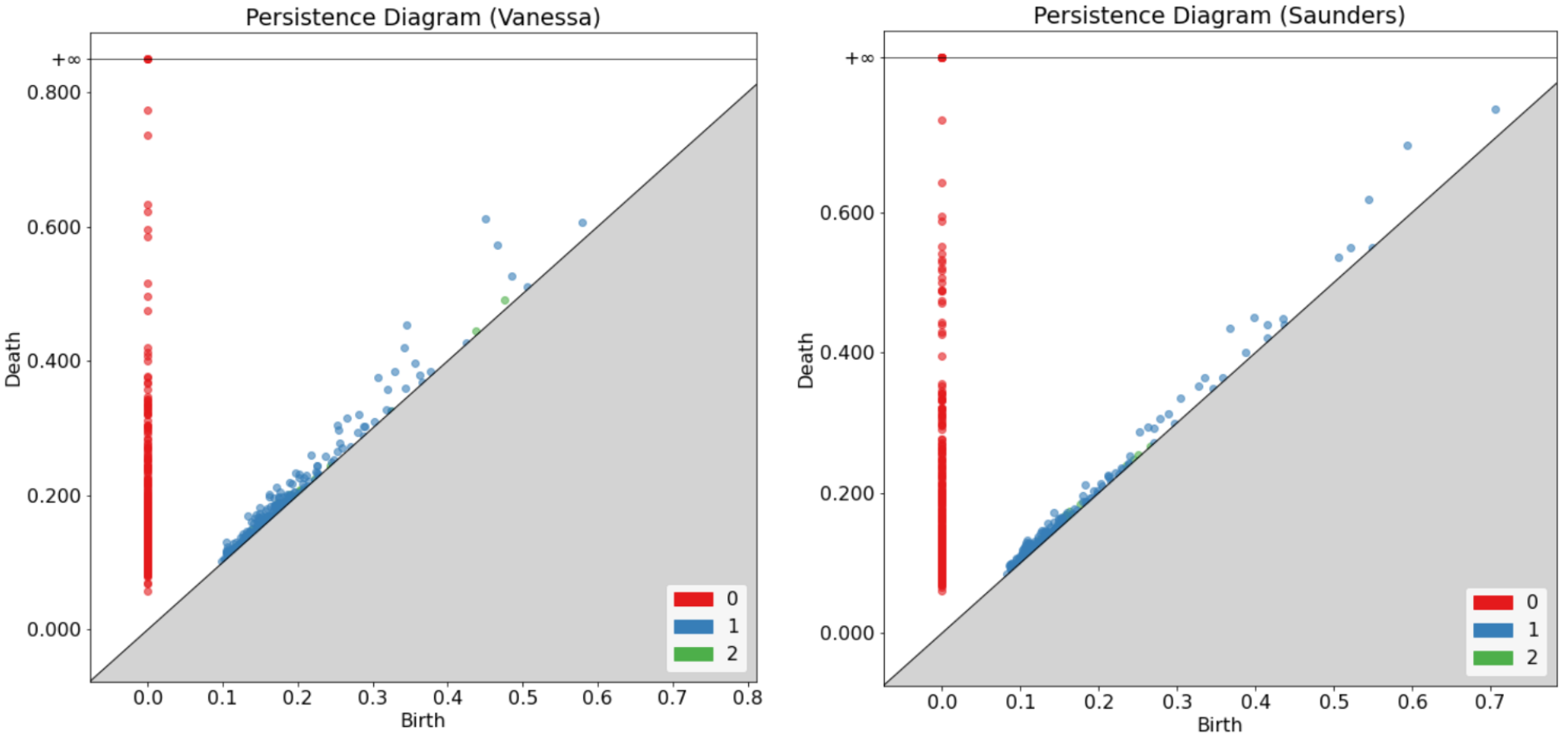
Now we plot the persistence diagrams of four selected test subjects which we have named for easy comparison. As you can see from the legend in the diagrams, the red dots represent the 0th homology, the blue dots represent the 1st homology, and the green dots represent the 2nd homology.

We also compare the barcode diagrams of our selected test subjects down below.

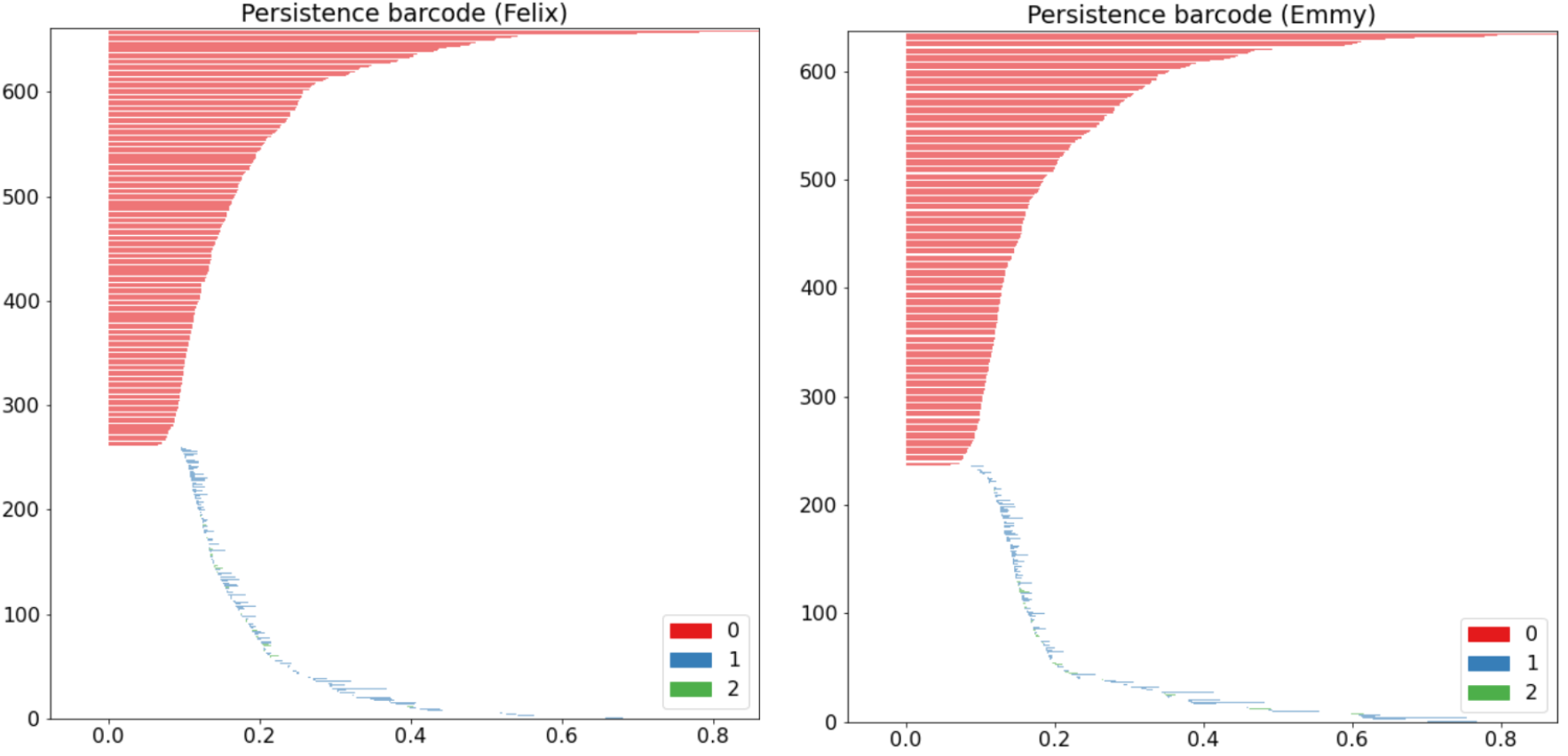
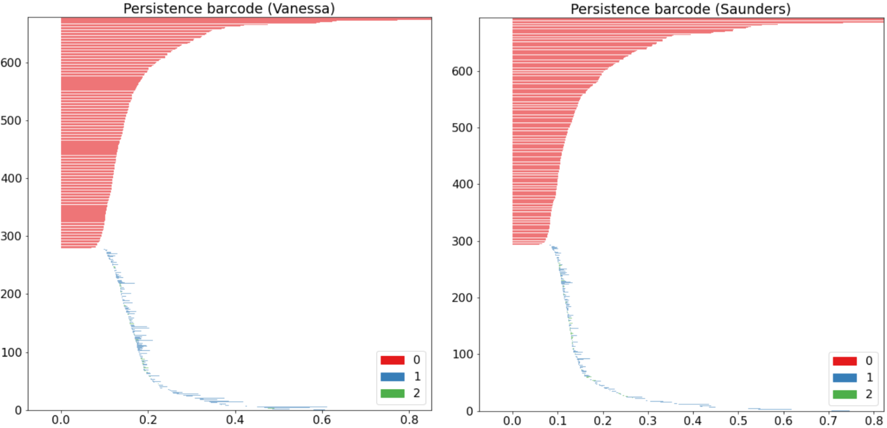
We especially note the variations in the outliers between each subject persistence diagrams. We can also see the disparities in the way each barcode diagram tapers off. While these figures allow us to easily observe the differences between typing patterns visually, we also utilized bottleneck distances to quantify these contrasts. Shown below are the bottleneck distances between each of our selected subjects in terms of the 0th, 1st, and 2nd homology.

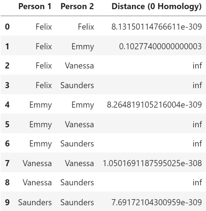
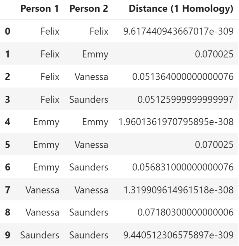
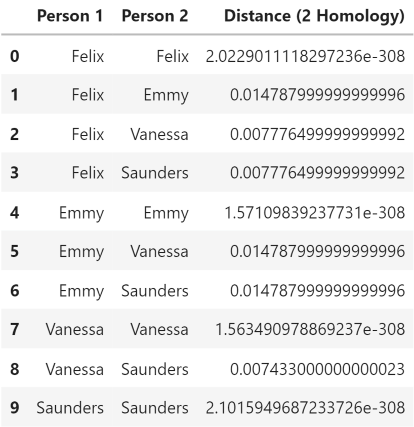
Across all different homologies, each subject has the smallest bottleneck distances with themselves by far. These bottleneck distances also span a small range as well. These are all indications that the slight differences displayed in the diagrams above are significant and detectable.

Results and Discussion of Future Work

We continued on by using bottleneck distance as our metric and implementing a grid search algorithm to optimize our hyperparameters. Note that we only kept the finite from our persistence intervals using the DiagramSelector. We then varied the epsilon (which represents the absolute error tolerated on the distance), n_neighbors (which represents the number of neighbors our k-nearest neighbors classifier uses), weights (which represent the how the nearest neighbors are weighted), and p (which represents the power for the Minkowski metric, 1 for Manhattan distance and 2 for Euclidean distance). Below is the optimized hyperparameter set found by our grid search algorithm.

  'Estimator__n_neighbors': 3,
  'Estimator__p': 1,
  'Estimator__weights': 'distance',
  'Scaler__use': False,
  'TDA__epsilon': 0.001

Our best model was able to correctly match the typing data in the training set to its corresponding test subject with 100% accuracy. However, the algorithm fails to generalize to cases outside of the training set, with accuracy dropped down to about 10%. We then considered Persistance Image as another possible metric and were able to increase our predication accuracy significantly with minimal tuning.

  Bottleneck distance training accuracy	= 100.0%
  Bottleneck distance prediction accuracy	= 9.803921568627452%
  Persistence Image prediction accuracy 	= 28.431372549019606%

With only 50 data points per persistence diagram, our dataset was on the smaller side in terms of topological data analysis. It is likely that we would have been able to achieve better results with more data points per diagram. In our future research, we also hope to explore other tools in topological data analysis that could lead to greater results, such as the Persistence Landscape, Sliced Wasserstein Kernel, and Persistence Weighted Gaussian Kernel.

References
  1. Title image created from Kolosov, K. (2022). Side view of faceless female typing on laptop sitting by table in evening in dark. Shutterstock. https://www.shutterstock.com/video/clip-22414081-side-view-faceless-female-typing-on-laptop
  2. Images and Gifs in "What is Persistent Homology?" Section are created from:
   i. Introduction to Persistent Homology. (2015, July 3). [Video]. YouTube. https://www.youtube.com/watch?v=h0bnG1Wavag&t=377s&ab_channel=MatthewWright
   ii. Koplik, G. (2022, May 30). Persistent Homology: A Non-Mathy Introduction with Examples. Medium. https://towardsdatascience.com/persistent-homology-with-examples-1974d4b9c3d0
   iii. Xu, X., Cisewski-Kehe, J., Green, S., & Nagai, D. (2019). Finding cosmic voids and filament loops using topological data analysis. Astronomy and Computing, 27, 34–52. https://doi.org/10.1016/j.ascom.2019.02.003